How to Get Normally Distributed Random Numbers With NumPy
Probability distributions describe the likelihood of all possible outcomes of an event or experiment. The normal distribution is one of the most useful probability distributions because it models many natural phenomena very well. With NumPy, you can create random number samples from the normal distribution.
This distribution is also called the Gaussian distribution or simply the bell curve. The latter hints at the shape of the distribution when you plot it:
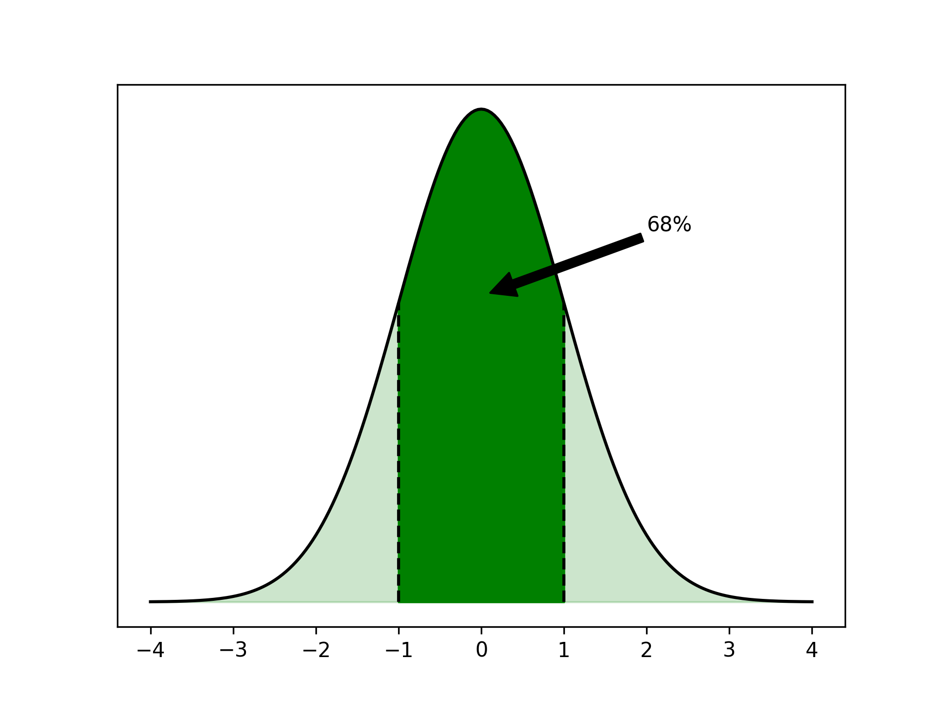
The normal distribution is symmetrical around its peak. Because of this symmetry, the mean of the distribution, often denoted by μ, is at that peak. The standard deviation, σ, describes how spread out the distribution is.
If some samples are normally distributed, then it’s probable that a random sample has a value close to the mean. In fact, about 68 percent of all samples are within one standard deviation of the mean.
You can interpret the area under the curve in the plot as a measure of probability. The darkly colored area, which represents all samples less than one standard deviation from the mean, is 68 percent of the full area under the curve.
- Arts
- Business
- Computers
- Games
- Health
- Home
- Kids and Teens
- Money
- News
- Personal Development
- Recreation
- Regional
- Reference
- Science
- Shopping
- Society
- Sports
- Бизнес
- Деньги
- Дом
- Досуг
- Здоровье
- Игры
- Искусство
- Источники информации
- Компьютеры
- Личное развитие
- Наука
- Новости и СМИ
- Общество
- Покупки
- Спорт
- Страны и регионы
- World